PhD on Synaptic Learning for Neuromorphic Vision

After over five years of researching in the field of biological learning for robotics, I have successfully completed my PhD. The full dissertation is published on the KIT bibliothek. In this blog post, I introduce the field of neuromorphic computing in layman’s terms, and present some of the results.

Silicon retina for a silicon brain

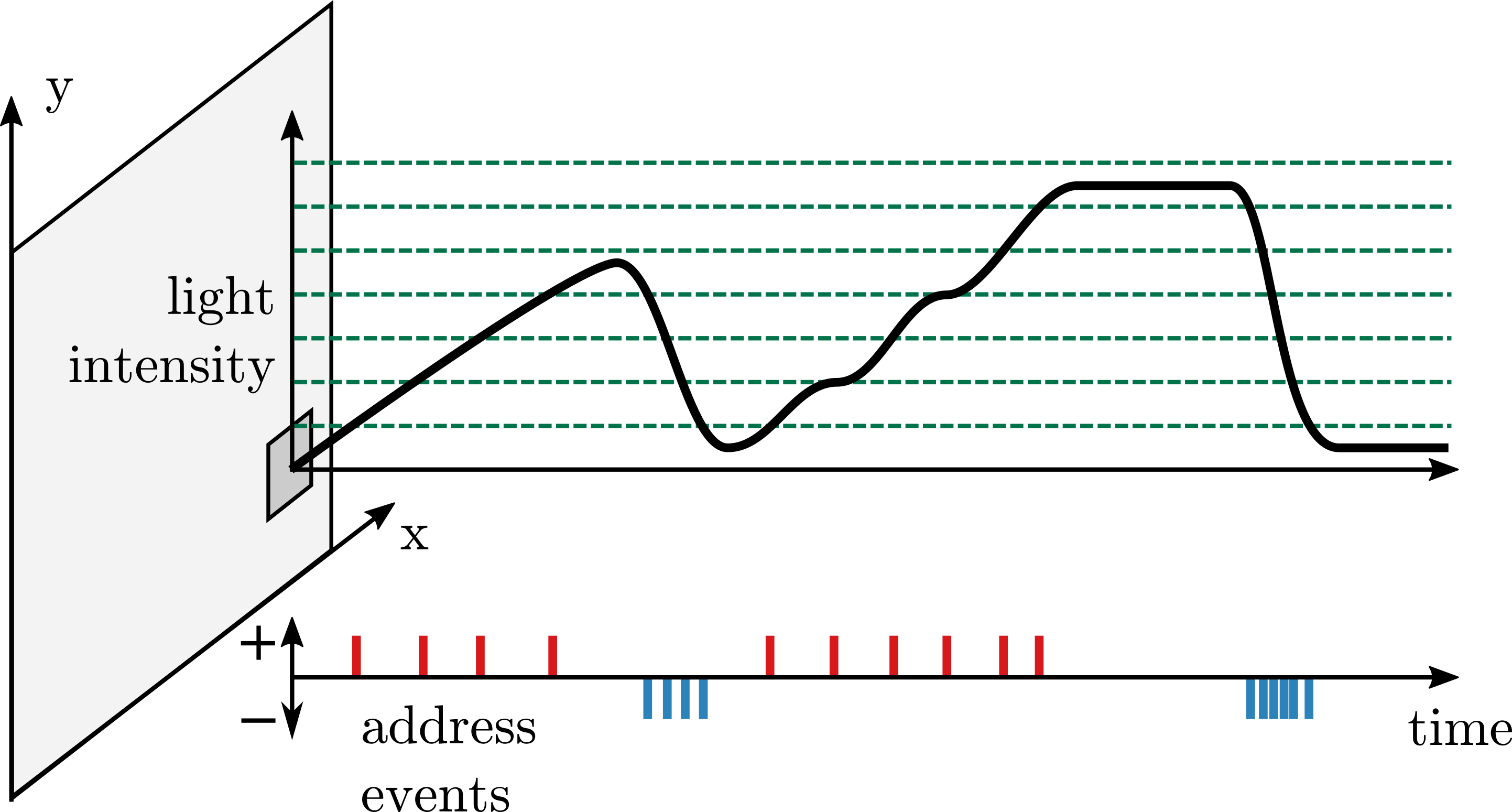
The Dynamic Vision Sensor is a very special type of camera. Conventional cameras take images at a given rate, around 30 times per seconds. Standard computer vision algorithms have to read and process these images, one by one. Modern smartphones are capable to perform such processing, but it consumes a lot of energy. On the other hand, the Dynamic Vision Sensor will only emit an individual event, when the light received by one pixel has changed. An event consists of the address of the pixel which changed, and whether light increased or decreased for this pixel. In other words, when the scene does not change, and the sensor does not move, no events are emitted. A computer vision algorithm can now run more efficiently: instead of processing full images regularly, it only has to process individual events, when the scene changes.

How the Dynamic Vision Sensor works

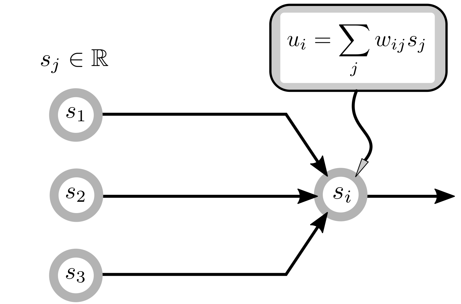
Until now, most computer vision algorithms were tailored to process images, not events. This also includes deep neural networks, which are used today in almost every computer vision problems. A deep neural network consists of neurons connected to each other in layers. Every neuron has a value, which is computed from the neurons in the previous layers and communicated to the neurons in the next layer. The actual computations depends on some values, called weights, which are learned. To process an image, the neurons of the first layer simply take the value of the pixels in the image. The values are used to compute the activation of the second layer of neurons and so on, until the last layer of neuron which is the output. Therefore, for every processed image, all neurons of a layer have to communicate their values synchronously. This is another expensive process (although it fits the GPU very well).

Conventional deep learning neuron

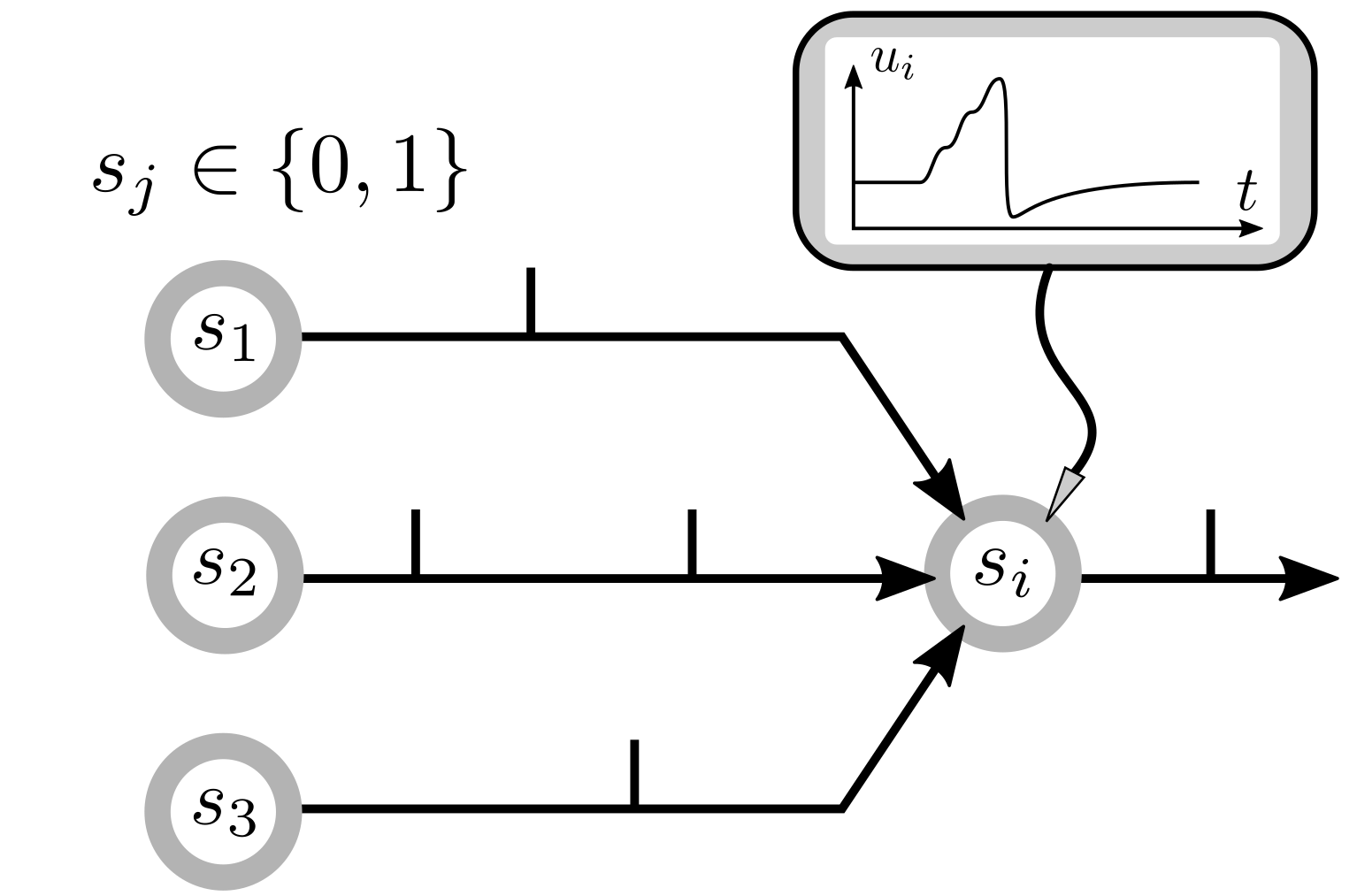
Spiking neurons are biologically-plausible version of conventional artificial neurons. They are particularly suited to processing events rather than images. Unlike a conventional neuron, a spiking neuron maintains a dynamical state which is not communicated to other neurons. Communication between neurons only consists of spikes, emitted when the state reaches a threshold. Spikes are spontaneous, stereotypical events: the information resides in the time at which the spike was emitted. Spikes and address events from the Dynamic Vision Sensors are very similar. In fact, to process address events with a spiking network, the first layer of neurons simply emit spikes for every address event.

Spiking neuron

Intuitively, processing a stream of events with a spiking network requires far less computations/communication than processing a sequence of images with conventional neural networks. The reason is, instead of processing the full information about the visual scene at every time-step again and again, we only process and communicate differences. Less computations implies potentially saving energy while running faster. However, this style of event-based computations do not fit conventional hardware very well: it is a paradigm shift. Taking advantage of these saved computations requires dedicated hardware, called neuromorphic hardware. Designing and manufacturing neuromorphic hardware was initiated in academia (Caltech, Zürich, Manchester, Dresden, …). Since then, both Intel and IBM started developing neuromorphic chips.

Deep learning networks are used everywhere today, because they can be easily trained with an algorithm called backpropagation. But how can deep networks of spiking neurons be trained? Are such networks capable of learning directly from the events of the Dynamic Vision Sensor? These are research questions I have investigated as part of my PhD.

Gradient descent in spiking networks

Over all the methods I have evaluated during my research, approximations of backpropagation turned out to provide the best performance. Not only was it learning more accurately, these approximations also solve some of the biologically implausible aspects of backpropagation, yielding a new theory of learning in the brain.

To go further, let’s formalize what is learning. Machine learning is a neat technique to solve complex problems, whenever data is available. At its core, learning requires:

• a parameterized model: some mathematical operations, which is a function of some parameters. In deep learning, the neural network is the model, which is parameterized by the synaptic weights \(W\).
• a loss function \(L: \mathbb{R}^n \rightarrow \mathbb{R}\), a metric assessing the performance of the synaptic weights on the task, using the available data. The goal of learning is to find the weights which minimize this loss function: \(W^\star=argmin_W L(W)\).

To find the best weights, a naive approach would be to try random weights, evaluate the loss function, and simply keep the ones where the loss function is the smallest. This is the strategy of black-box optimization methods such as evolutionary algorithms. However, evaluating the loss function is expensive, and we would like to do it as few times as possible. To this end, the best method to date is gradient descent. The gradient of the loss by the weights \(\frac{\partial L}{\partial w_{ij}}\) for all weights \(w_{ij} \in W\) is computed at the same time the loss \(L(W)\) is evaluated. Unlike black-box optimization, this requires to know what computations are performed by the model. By definition, the gradient of the loss by a weight \(w_{ij}\) means how an infinitesimal change in \(w_{ij}\) affects the loss. Therefore, by taking an (arbitrary small) step in the opposite direction of the gradient, we have good chances that the loss function will decrease. Gradient descent repeats this operation for all weights \(w_{ij} \in W\) until the loss function stops decreasing:

with \(\alpha \in \mathbb{R}\) the learning rate: an arbitrary small step.

Now back to neural networks. Backpropagation is the method used to compute the gradient \(\frac{\partial L}{\partial w_{ij}}\) in deep learning. To explain how it works, we need to dive in the equations of artificial neurons. A conventional deep learning neuron starts by summing up the values of its pre-synaptic neurons, weighted by the synaptic weights. It then applies a non-linear function, usually simply nulling-out negative values (ReLU). These are the \(u_i\) and the \(s_i\) terms in the following neural equations:

Using this definition, the step from a conventional neuron to a spiking neuron is small. In fact, there are only two important differences with spiking neurons:

• \(u_i\) carries a trace of the previous activity (it is a state which needs to be stored and updated). It is called the membrane potential.
• \(s_i\) is either 0 or 1, denoting spike and absence of spike, unlike conventional neuron which have output in \(\mathbb{R}\)).

Mathematically, a spiking neuron can be expressed as:

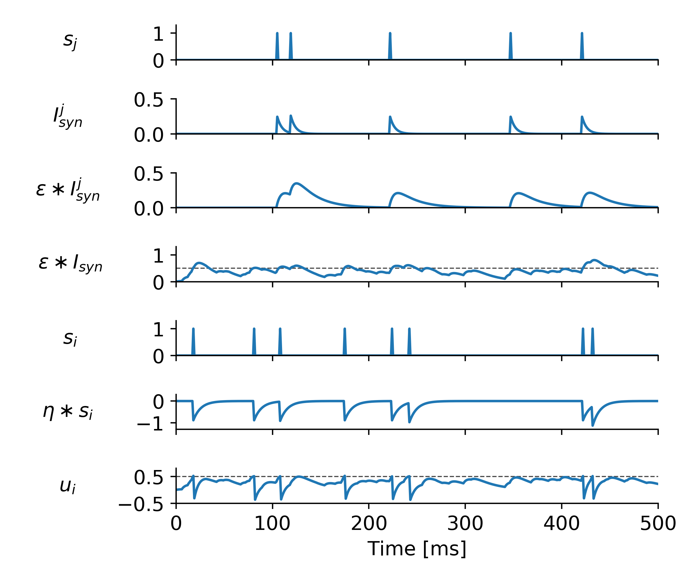
The \(\ast\) operation denotes a temporal convolution, with kernel \(\epsilon\) and \(\eta\) respectively. In words, this means that \(u_i\) also depends on the previous values of \(s_j\) and \(s_i\). A spike \(s_j\) is instantaneous, but it leaves a trace in \(u_i\): this is the first convolution. The second convolution denotes the decrease of the membrane potential of a neuron, right after it emitted a spike, commonly called the refractory period. A simple way to model this is simply by having the neuron inhibiting itself, with \(\eta \ast s_i < 0\).

Example dynamics of a spiking neuron

Let’s calculate the gradient \(\frac{\partial L}{\partial w_{ij}}\) for both an analog neuron and a spiking neuron. We can use the chain rule to express the gradient of a loss function $L$ with respect to the weight \(w_{ij}\):

Using this formulation, we see that the gradient is a multiplication of three terms. Let’s discuss these terms one by one.

Calculation of \(\dfrac{\partial u_i}{\partial w_{ij}}\):

This term captures how a change in synaptic weight affects the weighted sum of inputs $u_i$. For a conventional deep learning neuron, this term is simple to calculate, it is simply \(s_j\). For a spiking neuron, the calculation is more involved, especially because of how a change in weight \(w_{ij}\) affects the refractory period. Here comes the first approximation to backpropagation for spiking neuron: we ignore the refractory period in the gradient calculation. Note that if neurons do not spike often (in the brain neurons spike at maximum 60Hz) then refractory periods won’t play a big role in the dynamics. Therefore ignoring it in the gradient computation won’t affect learning too much. Using this approximation we can write \(\frac{\partial u_i}{\partial w_{ij}} \approx \epsilon \ast s_j\).

Calculation of \(\dfrac{\partial s_i}{\partial u_{i}}\):

This term captures how a change the membrane potential \(u_i\) affects spikes \(s_i\). With conventional deep learning neuron, this is simply the derivative of the ReLU function. For a spiking neuron however, the threshold function is not differentiable (it is undefined at the threshold value). Here comes the second approximation. We simply pretend that the threshold function was a similar, differentiable function – this is called a surrogate. For example, a function that linearly increases with slope \(1\) around the threshold value. We therefore have: \(\frac{\partial s_i}{\partial u_{i}} \approx 1\) around the threshold value, 0 otherwise.

Calculation of \(\dfrac{\partial L}{\partial s_i}\):

This term captures how a change in this neuron activity affects the loss of the whole network. The calculation of this term is the same for conventional neurons and spiking neurons. Note that \(s_i\) might not affect the loss directly if \(i\) is not an output neuron. Instead, it affects the activity of the neurons in the next layer, which themselves affect the next next layer, and so on until the output layer. Therefore, an exact computation of \(\frac{\partial L}{\partial s_i}\) also depends on the synaptic weights in the following layers. In conventional deep learning, this is not a big deal: when the error at the output layer becomes available, it is simply sent backward through the whole network. Hence the name backpropagation. For spiking networks, this is a problem: biological synpases are not bi-directional. This is where the third and last approximation jumps in. For spiking networks, we instantiate dedicated feedback synapses with random weights, distributing the network error to all neurons in all layers. This method is called feedback alignment, because the whole network will learn to align with the randomly chosen feedbacks. The actual choice of the loss function, and how feedback alignment is applied, is currently how modern synaptic learning rules for spiking networks differ.

Putting it all together

Injecting the three terms back into the gradient equation yields the synaptic learning rule for spiking neural networks:

with \(e_i\) the loss-dependent error. Like the dynamics of a spiking neuron, note that this gradient also has a temporal dynamics, due to the presence of the temporal convolution. In practice, this allows the spiking network to learn temporal correlations at no additional cost in memory, since the dynamical state for learning can be shared with the forward dynamics. Additionally, weight updates can be performed online, while sensory input is being streamed inside the network.

There are multiple instances of synaptic learning rules which relate to this derivation. As part of my PhD, we developed the DECOLLE learning rule [paper, code] together with Prof. Emre Neftci during a stay at the University of California, Irvine, funded by a DAAD scholarship. This learning rule achieves state-of-the-art accuracy on the popular gesture recognition dataset from IBM, DvsGesture. It is closely related to other rules such as SuperSpike and e-prop.

Conclusion

The CPU in your phone or laptop will not be replaced by a neuromorphic chip, but it might be complemented by it. Neuromorphic computing opens the door to novel applications where computing speed and low power consumption matters. With modern synaptic plasticity rules, such chips will also be capable of learning temporal correlations efficiently using approximations of gradient descent.